Plot Diagnostics for mixpoissonreg Objects — plot.mixpoissonreg • mixpoissonreg

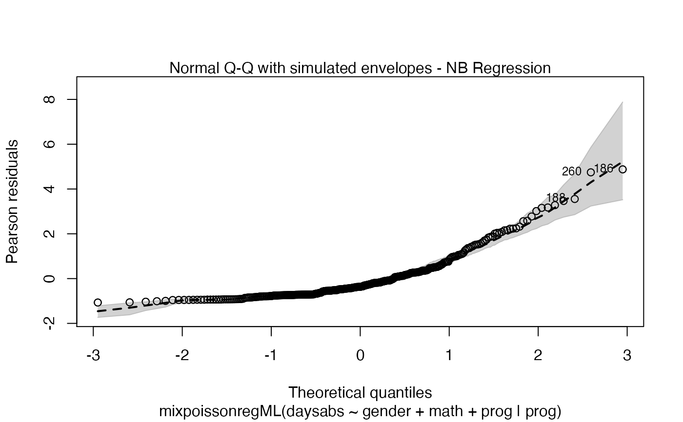
Currently there are six plots available. They contain residual analysis and global influence diagnostics. The plots are selectable by the which argument. The plots are: Residuals vs. obs. numbers; Normal Q-Q plots, which may contain simulated envelopes, if the fitted object has simulated envelopes; Cook's distances vs. obs. numbers; Generalized Cook's distances vs. obs. numbers; Cook's distances vs. Generalized Cook's distances; Response variables vs. fitted means. By default, the first two plots and the last two plots are provided.

# S3 method for mixpoissonreg
plot(
  x,
  which = c(1, 2, 5, 6),
  caption = list("Residuals vs Obs. number", "Normal Q-Q", "Cook's distance",
    "Generalized Cook's distance", "Cook's dist vs Generalized Cook's dist",
    "Response vs Fitted means"),
  sub.caption = NULL,
  qqline = TRUE,
  col.qqline = "black",
  main = "",
  line_col_env = "gray",
  line_col_median = "black",
  fill_col_env = "gray",
  fill_alpha_env = 0.7,
  ask = prod(graphics::par("mfcol")) < length(which) && grDevices::dev.interactive(),
  labels.id = names(stats::residuals(x)),
  label.pos = c(4, 2),
  type.cookplot = "h",
  id.n = 3,
  col.id = NULL,
  cex.id = 0.75,
  cex.oma.main = 1.25,
  cex.caption = 1,
  col.caption = "black",
  cex.points = 1,
  col.points = "black",
  include.modeltype = TRUE,
  include.residualtype = FALSE,
  ...
)

Arguments

x	object of class "mixpoissonreg" containing results from the fitted model. If the model was fitted with envelope = 0, the Q-Q plot will be produced without envelopes.
which	a list or vector indicating which plots should be displayed. If a subset of the plots is required, specify a subset of the numbers 1:6, see caption below for the different kinds. In plot number 2, 'Normal Q-Q', if the `mixpoissonreg` object was fitted with envelopes, a quantile-quantile plot with simulated envelopes will be displayed.
caption	captions to appear above the plots; character vector or list of valid graphics annotations. Can be set to "" or NA to suppress all captions.
sub.caption	common title-above the figures if there are more than one. If NULL, as by default, a possible abbreviated version of `deparse(x$call)` is used.
qqline	logical; if `TRUE` and the fit does not contain simulated envelopes, a qqline passing through the first and third quartiles of a standard normal distribution will be added to the normal Q-Q plot.
col.qqline	color of the qqline.
main	character; title to be placed at each plot additionally (and above) all captions.
line_col_env	line color for the upper and lower quantile curves of the simulated envelopes if the `mixpoissonreg` object was fitted with envelopes.
line_col_median	line color for the median curve of the simulated envelopes if the `mixpoissonreg` object was fitted with envelopes.
fill_col_env	fill color for the simulated envelopes if the `mixpoissonreg` object was fitted with envelopes.
fill_alpha_env	alpha of the envelope region, when the `mixpoissonreg` object was fitted with envelopes.
ask	logical; if `TRUE`, the user is asked before each plot.
labels.id	vector of labels, from which the labels for extreme points will be chosen. The default uses the observation numbers.
label.pos	positioning of labels, for the left half and right half of the graph respectively, for plots 2 and 6.
type.cookplot	character; what type of plot should be drawn for Cook's and Generalized Cook's distances (plots 3 and 4). The default is 'h'.
id.n	number of points to be labelled in each plot, starting with the most extreme.
col.id	color of point labels.
cex.id	magnification of point labels.
cex.oma.main	controls the size of the sub.caption only if that is above the figures when there is more than one.
cex.caption	controls the size of caption.
col.caption	controls the caption color.
cex.points	controls the size of the points.
col.points	controls the colors of the points.
include.modeltype	logical. Indicates whether the model type ('NB' or 'PIG') should be displayed on the captions.
include.residualtype	local. Indicates whether the name of the residual ('Pearson' or 'Score') should be displayed on the caption of plot 1 (Residuals vs. Index).
...	graphical parameters to be passed.

Value

It is called for its side effects.

Details

The plot method is implemented following the same structure as the plot.lm, so it will be easy to be used by practitioners that are familiar with glm objects.

These plots allows one to perform residuals analsysis and influence diagnostics. There are other global influence functions, see influence.mixpoissonreg.

See Barreto-Souza and Simas (2016), Cook and Weisberg (1982) and Zhu et al. (2001).

References

DOI:10.1007/s11222-015-9601-6 doi: 10.1007/s11222-015-9601-6 (Barreto-Souza and Simas; 2016)

Cook, D.R. and Weisberg, S. (1982) Residuals and Influence in Regression. (New York: Chapman and Hall, 1982)

Zhu, H.T., Lee, S.Y., Wei, B.C., Zhu, J. (2001) Case-deletion measures formodels with incomplete data. Biometrika, 88, 727–737.

Examples

# \donttest{
data("Attendance", package = "mixpoissonreg")

daysabs_fit <- mixpoissonreg(daysabs ~ gender + math +
prog | prog, data = Attendance)
plot(daysabs_fit, which = 1:6)

plot(daysabs_fit)

daysabs_fit_ml <- mixpoissonregML(daysabs ~ gender + math +
prog | prog, data = Attendance, envelope = 100)

plot(daysabs_fit_ml, which = 2)
# }

daysabs_prog <- mixpoissonreg(daysabs ~ prog, data = Attendance)
plot(daysabs_prog)

Plot Diagnostics for `mixpoissonreg` Objects

Arguments

Value

Details

References

See also

Examples