Mixed Poisson Regression for Overdispersed Count Data

Fits mixed Poisson regression models (Poisson-Inverse Gaussian or Negative-Binomial) on data sets with response variables being count data. The models can have varying precision parameter, where a linear regression structure (through a link function) is assumed to hold on the precision parameter. The Expectation-Maximization algorithm for both these models (Poisson Inverse Gaussian and Negative Binomial) is an important contribution of this package. Another important feature of this package is the set of functions to perform global and local influence analysis.

mixpoissonreg(
  formula,
  data,
  link.mean = c("log", "sqrt"),
  link.precision = c("identity", "log", "inverse.sqrt"),
  model = c("NB", "PIG"),
  method = c("EM", "ML"),
  residual = c("pearson", "score"),
  y = TRUE,
  x = TRUE,
  w = TRUE,
  envelope = 0,
  prob = 0.95,
  model.frame = TRUE,
  em_controls = list(maxit = 5000, em_tol = 10^(-5), em_tolgrad = 10^(-2)),
  optim_method = "L-BFGS-B",
  optim_controls = list()
)

mixpoissonreg.fit(
  x,
  y,
  w = NULL,
  link.mean = c("log", "sqrt"),
  link.precision = c("identity", "log", "inverse.sqrt"),
  model = c("NB", "PIG"),
  method = c("EM", "ML"),
  residual = c("pearson", "score"),
  envelope = 0,
  prob = 0.95,
  em_controls = list(maxit = 5000, em_tol = 10^(-5), em_tolgrad = 10^(-2)),
  optim_method = "L-BFGS-B",
  optim_controls = list()
)

Arguments

formula	symbolic description of the model (examples: `y ~ x1 + ... + xnbeta` and `y ~ x1 + ... + xnbeta \| w1 + ... + wnalpha`); see details below.
data	elements expressed in formula. This is usually a data frame composed by: (i) the observations formed by count data `z`, with z_i being non-negative integers, (ii) covariates for the mean submodel (columns `x1, ..., xnbeta`) and (iii) covariates for the precision submodel (columns `w1, ..., wnalphla`).
link.mean	optionally, a string containing the link function for the mean. If omitted, the 'log' link function will be used. The possible link functions for the mean are "log" and "sqrt".
link.precision	optionally, a string containing the link function the precision parameter. If omitted and the only precision covariate is the intercept, the 'identity' link function will be used, if omitted and there is a precision covariate other than the intercept, the 'log' link function will be used. The possible link functions for the precision parameter are "identity" and "inverse.sqrt" (which is $\phi^{-1/2} = w_i^T alpha$).
model	character ("NB" or "PIG") indicating the type of model to be fitted, with "NB" standing for Negative-Binomial and "PIG" standing for Poisson Inverse Gaussian. The default is "NB".
method	estimation method to be chosen between "EM" (Expectation-Maximization) and "ML" (Maximum-Likelihood). The default method is "EM".
residual	character indicating the type of residual to be evaluated ("pearson" or "score"). The default is "pearson". Notice that they coincide for Negative-Binomial models.
y	For `mixpoissonreg`: logical values indicating if the response vector should be returned as component. For `mixpoissonreg.fit`: a numerical vector of response variables with length `n`. Each coordinate must be a nonnegative-integer.
x	For `mixpoissonreg`: logical values indicating if the model matrix `x` should be returned as component. For `mixpoissonreg.fit`: a matrix of covariates with respect to the mean with dimension `(n,nbeta)`.
w	For `mixpoissonreg`: logical values indicating if the model matrix `w` should be returned as component. For `mixpoissonreg.fit` a matrix of covariates with respect to the precision parameter. The default is `NULL`. If not `NULL` must be of dimension `(n,nalpha)`.
envelope	number of simulations (synthetic data sets) to build envelopes for residuals (with `100*prob%` confidence level). The default `envelope = 0` dismisses the envelope analysis.
prob	probability indicating the confidence level for the envelopes (default: `prob` = 0.95). If `envelope` = 0, `prob` is ignored.
model.frame	logical indicating whether the model frame should be returned as component of the returned value.
em_controls	only used with the 'EM' method. A list containing two elements: `maxit` that contains the maximum number of iterations of the EM algorithm, the default is set to 5000; `em_tol` that defines the tolerance value to control the convergence criterion in the EM-algorithm, the default is set to 10^(-5); `em_tolgrad` that defines the tolerance value of the maximum-norm of the the gradient of the Q-function, the default is set to 10^(-2).
optim_method	main optimization algorithm to be used. The available methods are the same as those of `optim` function. The default is set to "L-BFGS-B".
optim_controls	a list of control arguments to be passed to the `optim` function in the optimization of the model. For the control options, see the 'Details' in the help of `optim` for the possible arguments.

Value

mixpoissonreg returns an object of class "mixpoissonreg" whereas mixpoissonreg.fit returns an object of class "mixpoissonreg_fit". Both objects are given by lists containing the outputs from the model fit (Negative-Binomial or Poisson Inverse Gaussian regression).

An object of the class "mixpoissonreg" is a list containing the following elements:

coefficients - a list with elements "mean" and "precision" containing the estimated coefficients of the model;
call - the formula used by the model. If using mixpoissonreg.fit, this returns NULL.
modelname - the fitted model, NB or PIG;
modeltype - the abbreviated model name
residualname - the name of the chosen residual in the call, 'pearson' or 'score';
niter - number of iterations of the EM algorithm if method = "EM" and number of iterations of the optim function, if method = "ML";
start - the initial guesses of the parameters
intercept - vector indicating if the intercept is present in the mean and/or in the precision regressions;
link.mean - link function of the mean;
link.precision - link function of the precision parameter;
fitted.values - a vector of fitted values in the response scale;
fitted.precisions - a vector of fitted precisions;
efron.pseudo.r2 - Efron's pseudo R^2: the squared correlation between the response variables and the predicted values;
vcov - covariance matrix of the parameters of the fitted model;
logLik - log-likelihood at the estimated parameters;
Qfunction - Q-function at the estimated parameters;
x - the covariates related to the mean (if x = TRUE);
w - the covariates related to the precision parameter (if w = TRUE);
y - the response variables (if y = TRUE);
model - if requested (the default), the model frame;
formula - the formula supplied;
nobs - number of observations
df.null - the residual degrees of freedom for the model with constant mean and constant precision;
df.residual - the residual degrees of freedom of the fitted model;
estimation_method - the estimation method, "EM" or "ML"
residuals - vector of raw residuals, that is, the response variable minus the fitted means;
std_errors - the standard errors of the estimated parameters;
envelope - the numerical envelopes used to build the Q-Q plot with simulated envelopes;
terms - (only for mixpoissonreg)the terms object used;
levels - (where relevant, only for mixpoissonreg) the levels of the factors used;
contrasts - (where relevant, only for mixpoissonreg) the contrasts used.

Details

Among the regression models with discrete response variables, Poisson regression is the most popular for modeling count data. See, for instance Sellers and Shmueli (2010). It is well-known that this model is equidispersed (that is, the mean is equal to the variance), which in practice may be an unrealistic assumption. Several models have been introduced in the literature to overcome this problem such as negative binomial (NB) and Poisson inverse gaussian (PIG) distributions (see Lawless, 1987). The most common way to do this is to consider a mixed Poisson distribution, which is defined as follows. Let $Z$ be a positive random variable (generally being continuous) with distribution function $G_{\tau}(\cdot)$, where $\tau$ denotes the parameter vector associated to the $G$ distribution. Let $Y|Z=z\sim$Poisson$(\mu z)$, for some constant $\mu>0$. Therefore $Y$ follows a mixed Poisson (MP) distribution with probability function given by $$P(Y=y)=\int_0^\infty\frac{e^{-\mu z}(\mu z)^y}{y!}dG_{\tau}(z),$$ for $y=0,1,\ldots$. With this, $Y$ has an overdispersed distribution and hence it is a natural alternative to the Poisson distribution. The most common choices for $Z$ are gamma and inverse-gaussian distributions, which yields $Y$ following, respectively, NB and PIG distributions. General properties of the MP distributions can be found in Karlis and Xekalaki (2005) and in the references therein.

In mixpoissonreg two regression models are implemented, namely, the NB and PIG regression models. We follow the definitions and notations given in Barreto-Souza and Simas (2016). The mixed Poisson regression model is defined by assuming $Y_1,\ldots,Y_n$ is a random sample where $Y_i\sim NB(\mu_i,\phi_i)$ or $Y_i\sim PIG(\mu_i,\phi_i)$ for $i = 1,\ldots,n$. Under this parameterization we have $E(Y_i) = \mu_i$ and $Var(Y_i) = \mu_i(1+\mu_i\phi_i^{-1}b''(\xi_0))$, where $b(\theta) = -\log(-\theta)$ and $\xi_0 = -1$ for the NB case, and $b(\theta) = -(-2\theta)^{1/2}$ and $\xi_0 = -1/2$ for the PIG case, with $b''(\cdot)$ being the second derivative of the function $b(\cdot)$. The following linear relations are assumed $$\Lambda_1(\mu_i) = x_i^T \beta$$ and $$\Lambda_2(\phi_i) = w_i^T \alpha,$$ where $\beta = (\beta_1,...,\beta_p)$ and $\alpha = (\alpha_1,...,\alpha_q)$ are real valued vectors. The terms $x_i^T$ and $v_i^T$ represent, respectively, the i-th row of the matrices "x" ($n\times p$) and "w" ($n\times q$) containing covariates in their columns ($x_{i,1}$ and $v_{i,1}$ may be 1 to handle intercepts).

Therefore, the mixpoissonreg package handles up to two regression structures at the same time: one for the mean parameter, one for the precision parameter. The regression structure for the mean is determined through a formula y ~ x1 + ... + xn, whereas the regression structure for the precision parameter is determined through the right-hand side of the formula using the separator "|". So, for example, a regression with x1,...,xn as covariates for the mean and z1,...,zm as covariates for the precision parameter corresponds to the formula y ~ x1 + ... + xn | z1 + ... + zm. If only there is only formula for the regression structure for the mean, the regression structure for the precision parameter will only have the intercept, that is, y ~ x1 + ... + xn is the same as y ~ x1 + ... + xn | 1.

In general, in this package, the EM-algorithm estimation method obtains estimates closer to the maximum likelihood estimate than the maximum likelihood estimation method, in the sense that the likelihood function evaluated at the EM-algorithm estimate is greater or equal (usually strictly greater) than the likelihood function evaluated at the maximum likelihood estimate. So, unless the processing time is an issue, we strongly recommend the EM-algorithm as the estimation method.

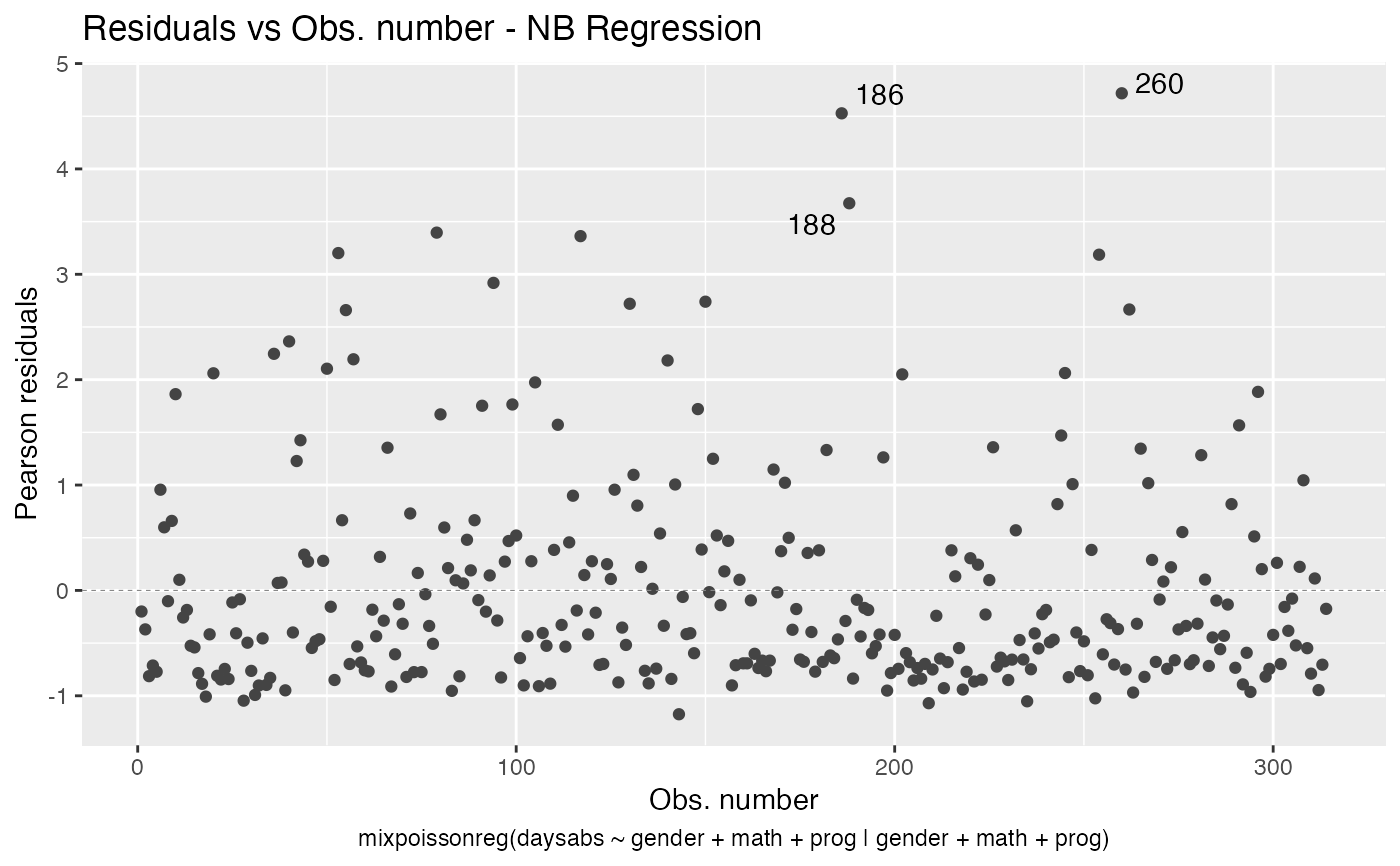
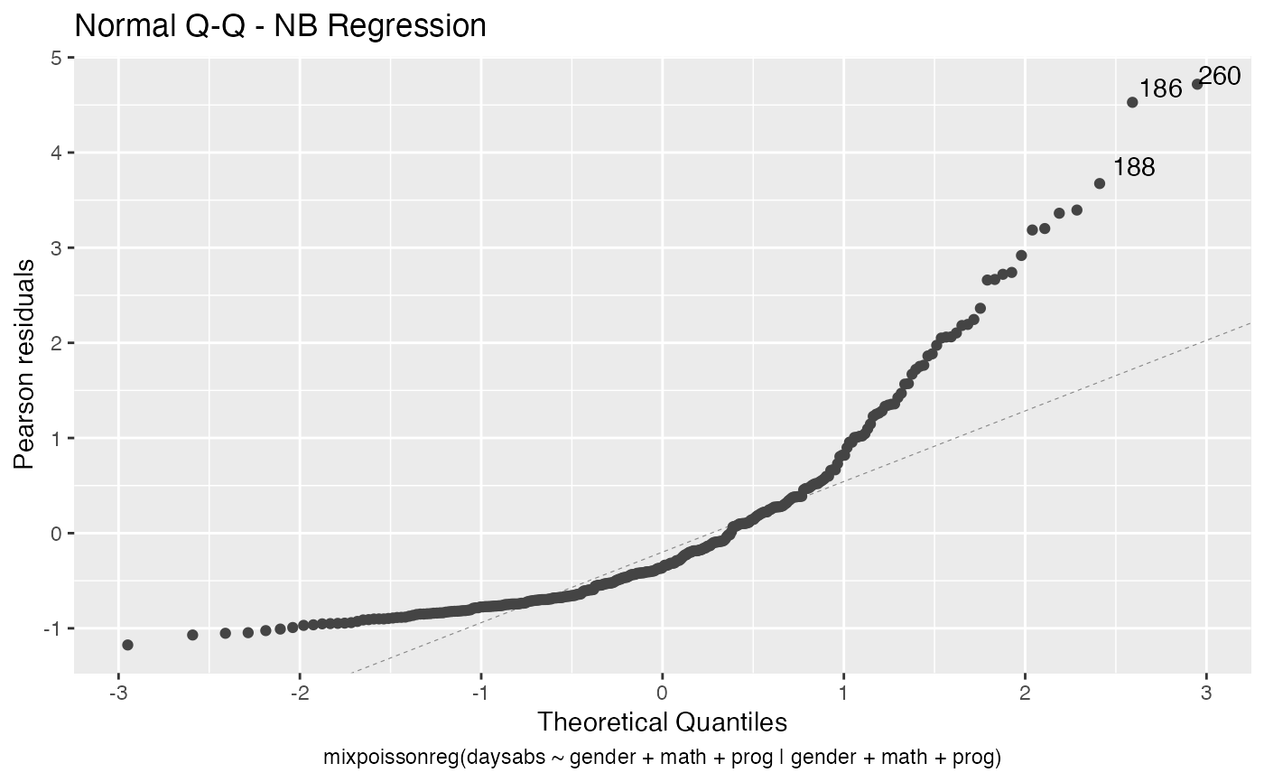
In Barreto-Souza and Simas (2016) two residuals were studied: the pearson residuals and the score residuals. Both these residuals are implemented in the mixpoissonreg package. They coincide for NB regression models. They can be accessed via the residuals method.

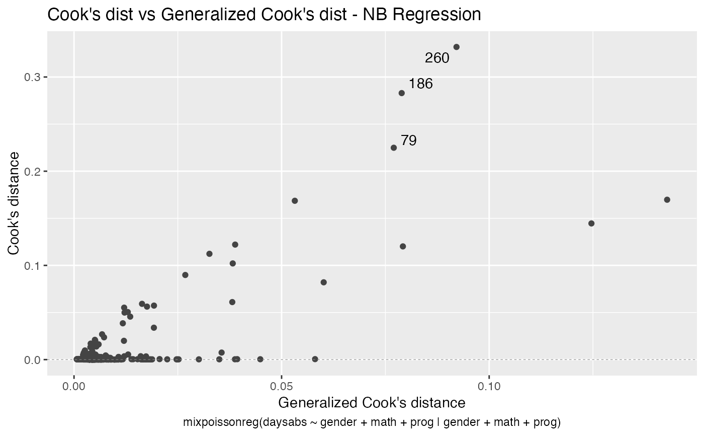
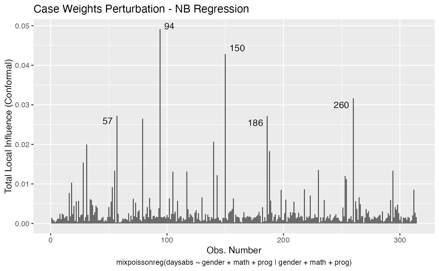
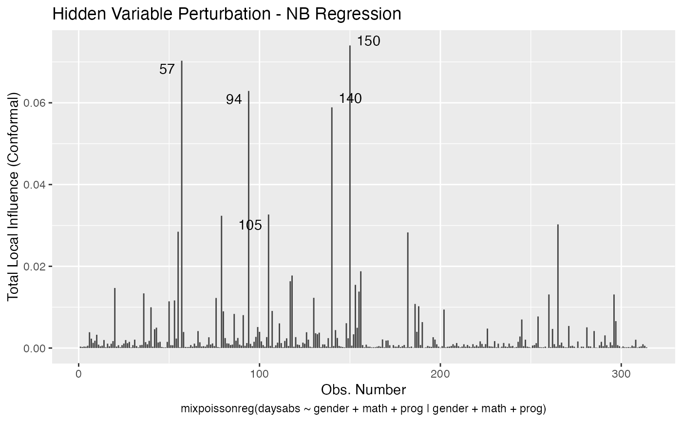
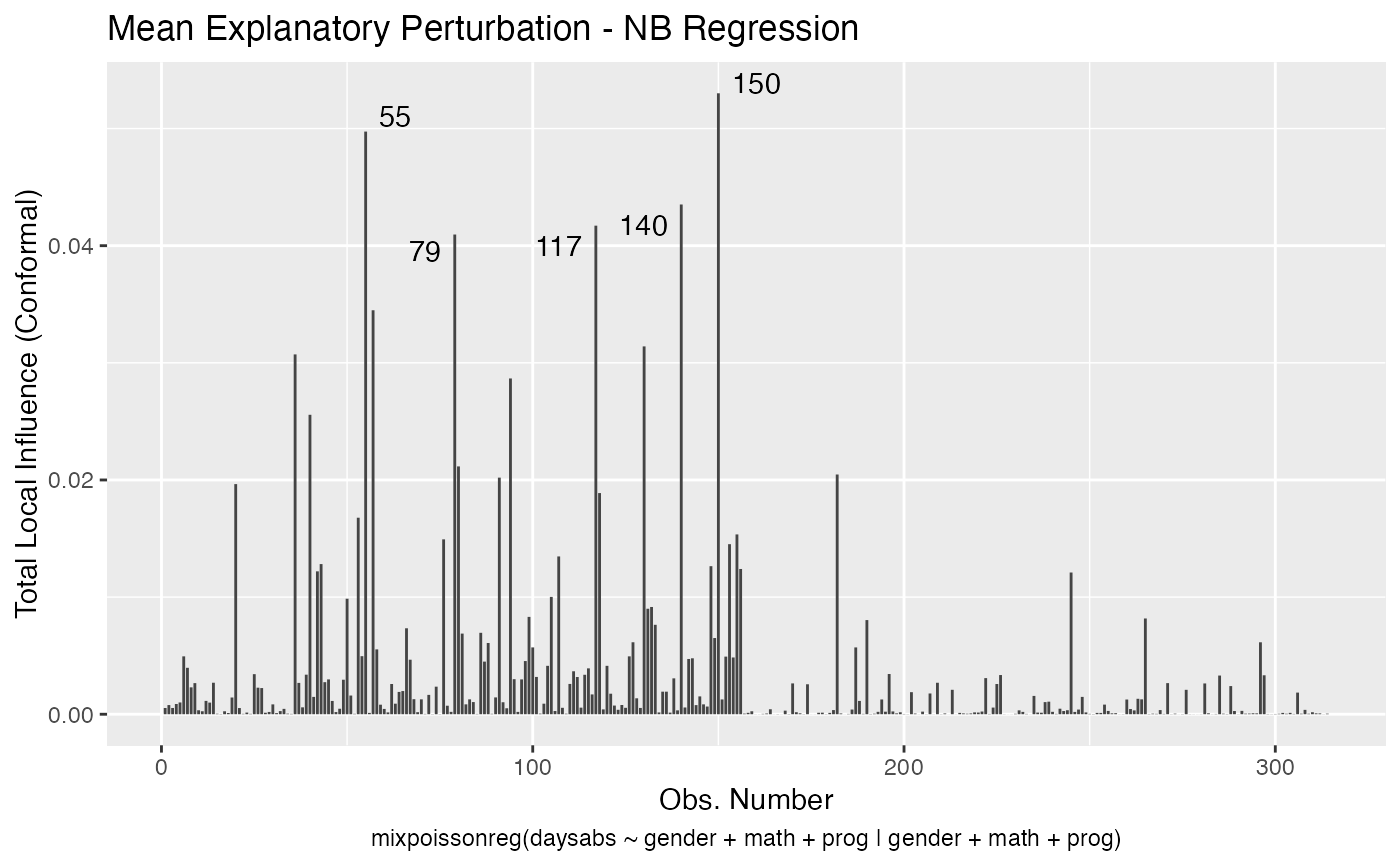
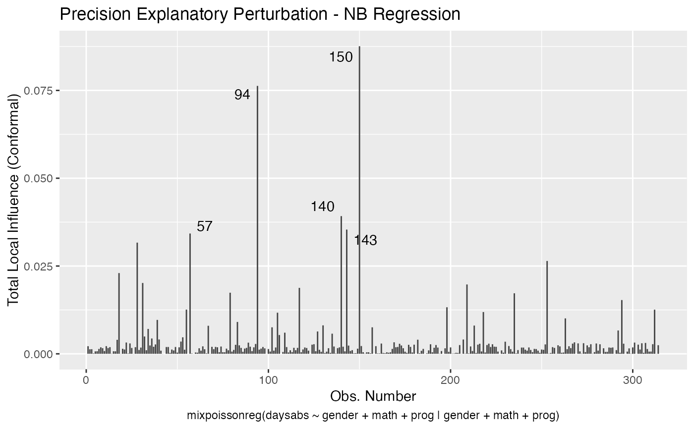
It is also noteworthy that all the global and local influence analysis tools developed in Barreto-Souza and Simas (2016) are implemented in this package. See influence.mixpoissonreg, local_influence.mixpoissonreg, local_influence_plot.mixpoissonreg and local_influence_autoplot.mixpoissonreg.

References

DOI:10.1007/s11222-015-9601-6 doi: 10.1007/s11222-015-9601-6 (Barreto-Souza and Simas; 2016)

URL:https://onlinelibrary.wiley.com/doi/abs/10.1111/j.1751-5823.2005.tb00250.x (Karlis and Xekalaki; 2005)

DOI:10.2307/3314912 doi: 10.2307/3314912 (Lawless; 1987)

Sellers, K.F. and Shmueli, G. (2010) A flexible regression model for count data. Ann. Appl. Stat., 4, 943-961

Examples

# Examples using the Attendance dataset:
# \donttest{
daysabs_fit <- mixpoissonreg(daysabs ~ gender + math +
prog | gender + math + prog, data = Attendance)
summary(daysabs_fit)
#> 
#> Negative Binomial Regression - Expectation-Maximization Algorithm
#> 
#> Call:
#> mixpoissonreg(formula = daysabs ~ gender + math + prog | gender + 
#>     math + prog, data = Attendance)
#> 
#> 
#> Pearson residuals:
#>      RSS      Min       1Q   Median       3Q      Max 
#> 322.0142  -1.1751  -0.6992  -0.3600   0.3014   4.7178 
#> 
#> Coefficients modeling the mean (with  link):
#>                 Estimate Std.error z-value Pr(>|z|)    
#> (Intercept)     2.746123  0.147412  18.629  < 2e-16 ***
#> gendermale     -0.245113  0.117967  -2.078  0.03773 *  
#> math           -0.006617  0.002317  -2.856  0.00429 ** 
#> progAcademic   -0.425983  0.132144  -3.224  0.00127 ** 
#> progVocational -1.269755  0.174444  -7.279 3.37e-13 ***
#> 
#> Coefficients modeling the precision (with  link):
#>                 Estimate Std.error z-value Pr(>|z|)    
#> (Intercept)     1.414227  0.343243   4.120 3.79e-05 ***
#> gendermale     -0.208397  0.203692  -1.023 0.306262    
#> math           -0.005123  0.004181  -1.225 0.220458    
#> progAcademic   -1.084418  0.305479  -3.550 0.000385 ***
#> progVocational -1.422051  0.343812  -4.136 3.53e-05 ***
#> ---
#> Signif. codes:  0 '***' 0.001 '**' 0.01 '*' 0.05 '.' 0.1 ' ' 1 
#> 
#> Efron's pseudo R-squared:  0.1860886 
#> Number of iterations of the EM algorithm = 11
# Base R plot of the fit
plot(daysabs_fit)
# ggplot2 plot of the fit
autoplot(daysabs_fit)
# plot of local influence measures
local_influence_plot(daysabs_fit)
# ggplot2 plot of local influence measures
local_influence_autoplot(daysabs_fit)
# Fitting a reduced model of the sabe type as the previous one
daysabs_fit_red <- mixpoissonreg(daysabs ~ gender + math +
prog | prog, data = Attendance, model = daysabs_fit$modeltype)
# Likelihood ratio test:
lmtest::lrtest(daysabs_fit, daysabs_fit_red)
#> Likelihood ratio test
#> 
#> Model 1: daysabs ~ gender + math + prog | gender + math + prog
#> Model 2: daysabs ~ gender + math + prog | prog
#>   #Df  LogLik Df  Chisq Pr(>Chisq)
#> 1  10 -853.20                     
#> 2   8 -854.41 -2 2.4077        0.3
# Wald test:
lmtest::waldtest(daysabs_fit, daysabs_fit_red)
#> Wald test
#> 
#> Model 1: daysabs ~ gender + math + prog | gender + math + prog
#> Model 2: daysabs ~ gender + math + prog | prog
#>   Res.Df Df  Chisq Pr(>Chisq)
#> 1    304                     
#> 2    306 -2 2.4149      0.299
# }

daysabs_prog <- mixpoissonreg(daysabs ~ prog, data = Attendance)
summary(daysabs_prog)
#> 
#> Negative Binomial Regression - Expectation-Maximization Algorithm
#> 
#> Call:
#> mixpoissonreg(formula = daysabs ~ prog, data = Attendance)
#> 
#> 
#> Pearson residuals:
#>      RSS      Min       1Q   Median       3Q      Max 
#> 340.4808  -0.9371  -0.6885  -0.2614   0.4086   5.2215 
#> 
#> Coefficients modeling the mean (with  link):
#>                Estimate Std.error z-value Pr(>|z|)    
#> (Intercept)      2.3656    0.1650  14.341  < 2e-16 ***
#> progAcademic    -0.4291    0.1845  -2.326     0.02 *  
#> progVocational  -1.3824    0.2000  -6.912 4.78e-12 ***
#> 
#> Coefficients modeling the precision (with  link):
#>             Estimate Std.error z-value Pr(>|z|)    
#> (Intercept)   1.0056    0.1023   9.832   <2e-16 ***
#> ---
#> Signif. codes:  0 '***' 0.001 '**' 0.01 '*' 0.05 '.' 0.1 ' ' 1 
#> 
#> Efron's pseudo R-squared:  0.1415831 
#> Number of iterations of the EM algorithm = 1