Analyzing overdispersed count data with the mixpoissonreg package
Wagner Barreto-Souza and Alexandre B. Simas
2021-03-12
Source:vignettes/tutorial-mixpoissonreg.Rmd
tutorial-mixpoissonreg.RmdDescription of the dataset
We will consider the dataset studied in Barreto-Souza and Simas (2016). The motivation for this study was to assess the attendance of high school students with respect to their gender, math score and which program they are enrolled. The data consists on 314 high school juniors from two urban high schools. The response variable, denoted by y, and the covariates of interest are:
y: number of days absent;
gender: sex (0=female and 1=male);
math: standardized math score for each student;
academic : indicator of academic program;
vocational: indicator of vocational program.
Model fitting and inference
It is well-known (see, for instance, https://stats.idre.ucla.edu/r/dae/negative-binomial-regression/) that the Poisson regression is not adequate for fitting this dataset. They also conclude that, when compared to the Poisson regression model, the Negative Binomial is more adequate. Therefore, this indicates that the data is overdispersed.
We will assume that the response variables \(Y_i\sim MP(\mu_i, \phi_i)\), that is, that each \(Y_i\) follows a mixed possion distribution with mean \(\mu_i\) and precision parameter \(\phi_i\).
We assume the following regression structures for the mean and precision parameters:
\[\log \mu_i = \beta_0 + \beta_1 {\tt gender}_i + \beta_2 {\tt math}_i + \beta_3 {\tt academic}_i + \beta_4 {\tt vocational}_i \] and
\[\log \phi_i = \alpha_0 + \alpha_1 {\tt gender}_i + \alpha_2 {\tt math}_i + \alpha_3 {\tt academic}_i + \alpha_4 {\tt vocational}_i.\] Let us fit this model under the assumption of Negative Binomial (NB) and Poisson Inverse Gaussian (PIG) distributions.
library(mixpoissonreg)

fit_nb_full <- mixpoissonreg(daysabs ~ gender + math + prog | gender + math + prog,
                             model = "NB", data = Attendance)

fit_pig_full <- mixpoissonreg(daysabs ~ gender + math + prog | gender + math + prog,
                             model = "PIG", data = Attendance)
The summary for the NB-regression fitting is:
summary(fit_nb_full)
#>
#> Negative Binomial Regression - Expectation-Maximization Algorithm
#>
#> Call:
#> mixpoissonreg(formula = daysabs ~ gender + math + prog | gender +
#>     math + prog, data = Attendance, model = "NB")
#>
#>
#> Pearson residuals:
#>      RSS      Min       1Q   Median       3Q      Max
#> 322.0142  -1.1751  -0.6992  -0.3600   0.3014   4.7178
#>
#> Coefficients modeling the mean (with  link):
#>                 Estimate Std.error z-value Pr(>|z|)
#> (Intercept)     2.746123  0.147412  18.629  < 2e-16 ***
#> gendermale     -0.245113  0.117967  -2.078  0.03773 *
#> math           -0.006617  0.002317  -2.856  0.00429 **
#> progAcademic   -0.425983  0.132144  -3.224  0.00127 **
#> progVocational -1.269755  0.174444  -7.279 3.37e-13 ***
#>
#> Coefficients modeling the precision (with  link):
#>                 Estimate Std.error z-value Pr(>|z|)
#> (Intercept)     1.414227  0.343243   4.120 3.79e-05 ***
#> gendermale     -0.208397  0.203692  -1.023 0.306262
#> math           -0.005123  0.004181  -1.225 0.220458
#> progAcademic   -1.084418  0.305479  -3.550 0.000385 ***
#> progVocational -1.422051  0.343812  -4.136 3.53e-05 ***
#> ---
#> Signif. codes:  0 '***' 0.001 '**' 0.01 '*' 0.05 '.' 0.1 ' ' 1
#>
#> Efron's pseudo R-squared:  0.1860886
#> Number of iterations of the EM algorithm = 11
For the PIG-regression, the summary is
summary(fit_pig_full)
#>
#> Poisson Inverse Gaussian Regression - Expectation-Maximization Algorithm
#>
#> Call:
#> mixpoissonreg(formula = daysabs ~ gender + math + prog | gender +
#>     math + prog, data = Attendance, model = "PIG")
#>
#>
#> Pearson residuals:
#>      RSS      Min       1Q   Median       3Q      Max
#> 239.2040  -1.0836  -0.6058  -0.3062   0.2519   4.1196
#>
#> Coefficients modeling the mean (with  link):
#>                 Estimate Std.error z-value Pr(>|z|)
#> (Intercept)     2.750853  0.165416  16.630  < 2e-16 ***
#> gendermale     -0.251161  0.136873  -1.835  0.06651 .
#> math           -0.006730  0.002679  -2.512  0.01202 *
#> progAcademic   -0.423484  0.148479  -2.852  0.00434 **
#> progVocational -1.260924  0.203436  -6.198 5.71e-10 ***
#>
#> Coefficients modeling the precision (with  link):
#>                 Estimate Std.error z-value Pr(>|z|)
#> (Intercept)     1.211252  0.438442   2.763 0.005734 **
#> gendermale     -0.114332  0.304682  -0.375 0.707475
#> math           -0.005686  0.006098  -0.932 0.351111
#> progAcademic   -1.284018  0.386350  -3.323 0.000889 ***
#> progVocational -1.610037  0.475613  -3.385 0.000711 ***
#> ---
#> Signif. codes:  0 '***' 0.001 '**' 0.01 '*' 0.05 '.' 0.1 ' ' 1
#>
#> Efron's pseudo R-squared:  0.1861608
#> Number of iterations of the EM algorithm = 2632
These summaries suggest that gender and math covariates are not significant to explain the precision parameter. So we will obtain fits for the NB and PIG regressions without these variables for the precision paramters, then we will perform Wald and likelihood-ratio tests to confirm that indeed they are not significant.
fit_nb_red <- mixpoissonreg(daysabs ~ gender + math + prog | prog,
                             model = "NB", data = Attendance)

fit_pig_red <- mixpoissonreg(daysabs ~ gender + math + prog | prog,
                             model = "PIG", data = Attendance)
Let us check the summaries for these regressions:
summary(fit_nb_red)
#>
#> Negative Binomial Regression - Expectation-Maximization Algorithm
#>
#> Call:
#> mixpoissonreg(formula = daysabs ~ gender + math + prog | prog,
#>     data = Attendance, model = "NB")
#>
#>
#> Pearson residuals:
#>      RSS      Min       1Q   Median       3Q      Max
#> 323.6673  -1.0659  -0.7203  -0.3656   0.3064   4.8768
#>
#> Coefficients modeling the mean (with  link):
#>                 Estimate Std.error z-value Pr(>|z|)
#> (Intercept)     2.752395  0.152504  18.048  < 2e-16 ***
#> gendermale     -0.257188  0.116905  -2.200  0.02781 *
#> math           -0.006792  0.002274  -2.987  0.00282 **
#> progAcademic   -0.423971  0.132284  -3.205  0.00135 **
#> progVocational -1.238556  0.173103  -7.155 8.37e-13 ***
#>
#> Coefficients modeling the precision (with  link):
#>                Estimate Std.error z-value Pr(>|z|)
#> (Intercept)      1.1124    0.2783   3.997 6.41e-05 ***
#> progAcademic    -1.0865    0.3074  -3.534 0.000409 ***
#> progVocational  -1.5211    0.3395  -4.480 7.45e-06 ***
#> ---
#> Signif. codes:  0 '***' 0.001 '**' 0.01 '*' 0.05 '.' 0.1 ' ' 1
#>
#> Efron's pseudo R-squared:  0.1861217
#> Number of iterations of the EM algorithm = 2453
and
summary(fit_pig_red)
#>
#> Poisson Inverse Gaussian Regression - Expectation-Maximization Algorithm
#>
#> Call:
#> mixpoissonreg(formula = daysabs ~ gender + math + prog | prog,
#>     data = Attendance, model = "PIG")
#>
#>
#> Pearson residuals:
#>      RSS      Min       1Q   Median       3Q      Max
#> 239.2879  -1.0042  -0.6101  -0.3107   0.2734   4.2814
#>
#> Coefficients modeling the mean (with  link):
#>                 Estimate Std.error z-value Pr(>|z|)
#> (Intercept)     2.805150  0.162182  17.296  < 2e-16 ***
#> gendermale     -0.282333  0.122772  -2.300  0.02147 *
#> math           -0.007770  0.002398  -3.240  0.00120 **
#> progAcademic   -0.422885  0.148013  -2.857  0.00428 **
#> progVocational -1.215877  0.197264  -6.164 7.11e-10 ***
#>
#> Coefficients modeling the precision (with  link):
#>                Estimate Std.error z-value Pr(>|z|)
#> (Intercept)      0.9277    0.3308   2.805 0.005039 **
#> progAcademic    -1.2799    0.3853  -3.322 0.000894 ***
#> progVocational  -1.7440    0.4506  -3.870 0.000109 ***
#> ---
#> Signif. codes:  0 '***' 0.001 '**' 0.01 '*' 0.05 '.' 0.1 ' ' 1
#>
#> Efron's pseudo R-squared:  0.1858037
#> Number of iterations of the EM algorithm = 19
Now, let us perform a Wald test:
lmtest::waldtest(fit_nb_red, fit_nb_full)
#> Wald test
#>
#> Model 1: daysabs ~ gender + math + prog | prog
#> Model 2: daysabs ~ gender + math + prog | gender + math + prog
#>   Res.Df Df  Chisq Pr(>Chisq)
#> 1    306
#> 2    304  2 2.4149      0.299
and
lmtest::waldtest(fit_pig_red, fit_pig_full)
#> Wald test
#>
#> Model 1: daysabs ~ gender + math + prog | prog
#> Model 2: daysabs ~ gender + math + prog | gender + math + prog
#>   Res.Df Df  Chisq Pr(>Chisq)
#> 1    306
#> 2    304  2 0.9304      0.628
Now, let us perform likelihood tests:
lmtest::lrtest(fit_nb_red, fit_nb_full)
#> Likelihood ratio test
#>
#> Model 1: daysabs ~ gender + math + prog | prog
#> Model 2: daysabs ~ gender + math + prog | gender + math + prog
#>   #Df  LogLik Df  Chisq Pr(>Chisq)
#> 1   8 -854.41
#> 2  10 -853.20  2 2.4077        0.3
and
lmtest::lrtest(fit_pig_red, fit_pig_full)
#> Likelihood ratio test
#>
#> Model 1: daysabs ~ gender + math + prog | prog
#> Model 2: daysabs ~ gender + math + prog | gender + math + prog
#>   #Df  LogLik Df  Chisq Pr(>Chisq)
#> 1   8 -857.52
#> 2  10 -857.05  2 0.9507     0.6217
The above tests indicate that, indeed, gender and math are not significant for the precision parameter. So we will work with the reduced models.
Let us also build a small data frame containing the estimated mean, \(\widehat{\mu}\), for some combinations of the covariates. First for the NB regression model:
library(tidyr)
library(dplyr)
#>
#> Attaching package: 'dplyr'
#> The following objects are masked from 'package:stats':
#>
#>     filter, lag
#> The following objects are masked from 'package:base':
#>
#>     intersect, setdiff, setequal, union

gender <- c("female", "male")
prog <- c("Academic", "General", "Vocational")
math <- c(0, 99)

new_cov <- crossing(gender, prog, math)

pred_values_nb <- predict(fit_nb_red, newdata = new_cov)

bind_cols(new_cov, "Predicted_Means_NB" = pred_values_nb)
#> # A tibble: 12 x 4
#>    gender prog        math Predicted_Means_NB
#>    <chr>  <chr>      <dbl>              <dbl>
#>  1 female Academic       0              15.7
#>  2 female Academic      99               8.00
#>  3 female General        0              10.3
#>  4 female General       99               5.24
#>  5 female Vocational     0               4.54
#>  6 female Vocational    99               2.32
#>  7 male   Academic       0              12.1
#>  8 male   Academic      99               6.19
#>  9 male   General        0               7.93
#> 10 male   General       99               4.05
#> 11 male   Vocational     0               3.51
#> 12 male   Vocational    99               1.79
Now for the PIG regression model:
pred_values_pig <- predict(fit_pig_red, newdata = new_cov)

bind_cols(new_cov, "Predicted_Means_PIG" = pred_values_pig)
#> # A tibble: 12 x 4
#>    gender prog        math Predicted_Means_PIG
#>    <chr>  <chr>      <dbl>               <dbl>
#>  1 female Academic       0               16.5
#>  2 female Academic      99                7.66
#>  3 female General        0               10.8
#>  4 female General       99                5.02
#>  5 female Vocational     0                4.90
#>  6 female Vocational    99                2.27
#>  7 male   Academic       0               12.5
#>  8 male   Academic      99                5.78
#>  9 male   General        0                8.17
#> 10 male   General       99                3.78
#> 11 male   Vocational     0                3.69
#> 12 male   Vocational    99                1.71
Residual analysis
Let us fit the reduced models with envelopes. To reduce computational cost, we will fit these models with the direct maximum likelihood estimation and with respect to the Pearson residual.
set.seed(2021)
# We are fixing the seed for reproducibility
fit_nb_red_env <- mixpoissonregML(daysabs ~ gender + math + prog | prog,
                             model = "NB", data = Attendance, envelope = 100)

fit_pig_red_env <- mixpoissonregML(daysabs ~ gender + math + prog | prog,
                             model = "PIG", data = Attendance, envelope = 100)
Let us check the coverage of the envelopes for the NB fit:
summary(fit_nb_red_env)
#>
#> Negative Binomial Regression - Maximum-Likelihood Estimation
#>
#> Call:
#> mixpoissonregML(formula = daysabs ~ gender + math + prog | prog,
#>     data = Attendance, model = "NB", envelope = 100)
#>
#>
#> Pearson residuals:
#>      RSS      Min       1Q   Median       3Q      Max
#> 323.9340  -1.0684  -0.7203  -0.3660   0.3062   4.8766
#>
#> Coefficients modeling the mean (with  link):
#>                 Estimate Std.error z-value Pr(>|z|)
#> (Intercept)     2.752203  0.152251  18.077  < 2e-16 ***
#> gendermale     -0.256901  0.116816  -2.199  0.02786 *
#> math           -0.006791  0.002271  -2.989  0.00279 **
#> progAcademic   -0.423978  0.132089  -3.210  0.00133 **
#> progVocational -1.238641  0.172941  -7.162 7.94e-13 ***
#>
#> Coefficients modeling the precision (with  link):
#>                Estimate Std.error z-value Pr(>|z|)
#> (Intercept)      1.1185    0.2784   4.017 5.88e-05 ***
#> progAcademic    -1.0925    0.3075  -3.552 0.000382 ***
#> progVocational  -1.5270    0.3396  -4.496 6.91e-06 ***
#> ---
#> Signif. codes:  0 '***' 0.001 '**' 0.01 '*' 0.05 '.' 0.1 ' ' 1
#>
#> Efron's pseudo R-squared:  0.1861221
#> Percentage of residuals within the envelope = 97.4522
#> Number of function calls by 'optim' = 4
and for the PIG fit:
summary(fit_pig_red_env)
#>
#> Poisson Inverse Gaussian Regression - Maximum-Likelihood Estimation
#>
#> Call:
#> mixpoissonregML(formula = daysabs ~ gender + math + prog | prog,
#>     data = Attendance, model = "PIG", envelope = 100)
#>
#>
#> Pearson residuals:
#>      RSS      Min       1Q   Median       3Q      Max
#> 239.2987  -1.0042  -0.6101  -0.3107   0.2734   4.2816
#>
#> Coefficients modeling the mean (with  link):
#>                 Estimate Std.error z-value Pr(>|z|)
#> (Intercept)     2.805150  0.162182  17.296  < 2e-16 ***
#> gendermale     -0.282333  0.122772  -2.300  0.02147 *
#> math           -0.007771  0.002398  -3.240  0.00120 **
#> progAcademic   -0.422885  0.148011  -2.857  0.00428 **
#> progVocational -1.215877  0.197261  -6.164  7.1e-10 ***
#>
#> Coefficients modeling the precision (with  link):
#>                Estimate Std.error z-value Pr(>|z|)
#> (Intercept)      0.9277    0.3308   2.805 0.005038 **
#> progAcademic    -1.2799    0.3853  -3.322 0.000894 ***
#> progVocational  -1.7440    0.4506  -3.870 0.000109 ***
#> ---
#> Signif. codes:  0 '***' 0.001 '**' 0.01 '*' 0.05 '.' 0.1 ' ' 1
#>
#> Efron's pseudo R-squared:  0.1858035
#> Percentage of residuals within the envelope = 94.9045
#> Number of function calls by 'optim' = 6
By looking at both coverages, the assumption of the response following a mixed Poisson distribution seems reasonable. Furthermore, both regressions seem to provide adequate fit.
Also, notice that, even though the fits seem adequate, their Efron’s \(R^2\) are low, around 18%. This is due to the high overdispersion of the responses, together with the fact that the mean is not a good predictor for the response when using counting data. Therefore, for datasets with low Efron’s pseudo-\(R^2\), such as this one, we recommend to use the mode. We plan on providing a function from prediction based on the mode in the future.
Let us check the diagnostic plots of the NB fit
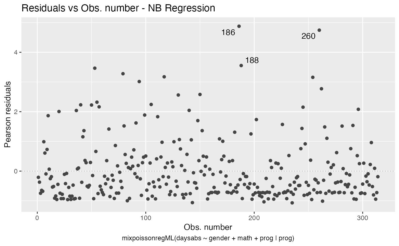
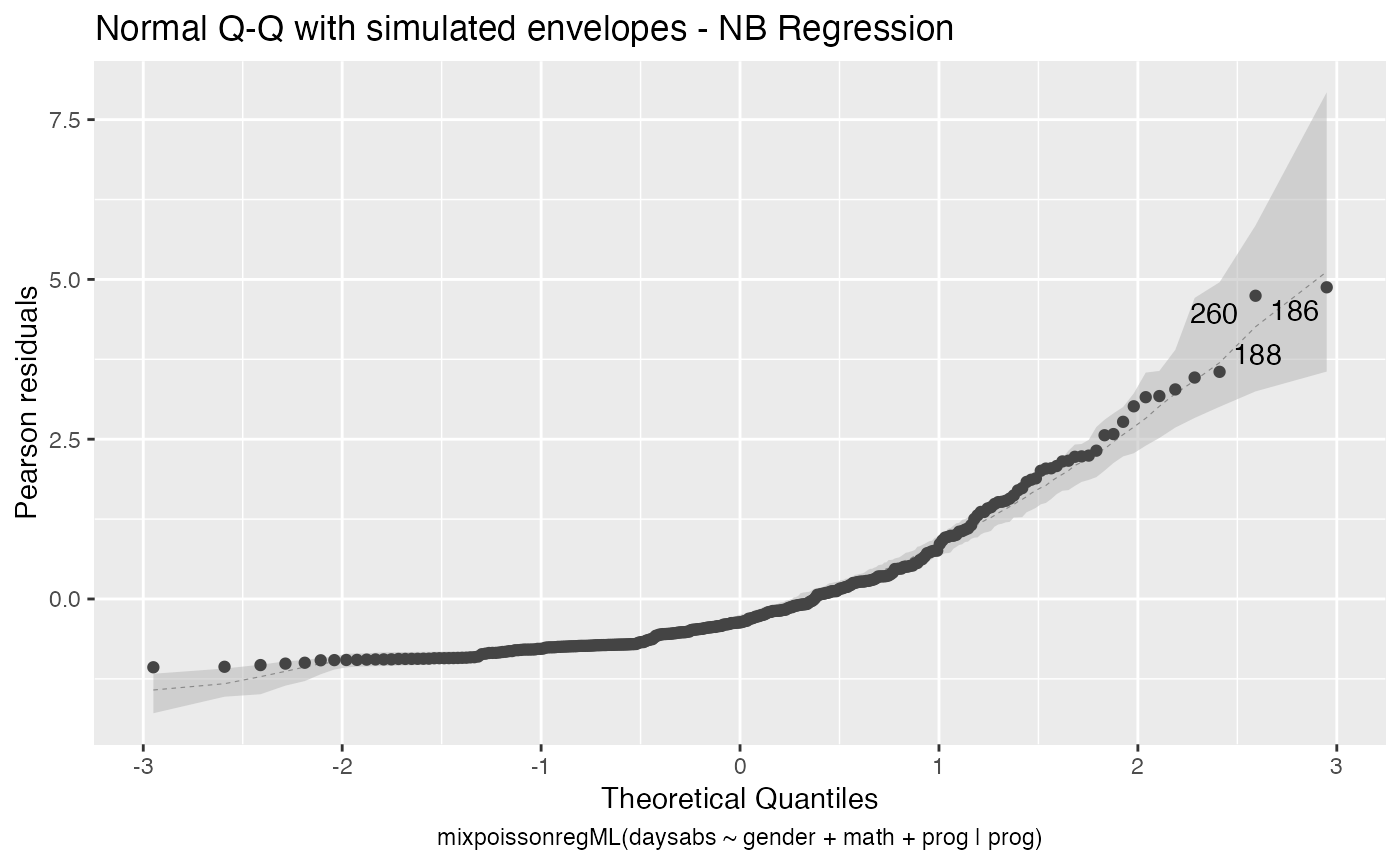
and for the PIG fit
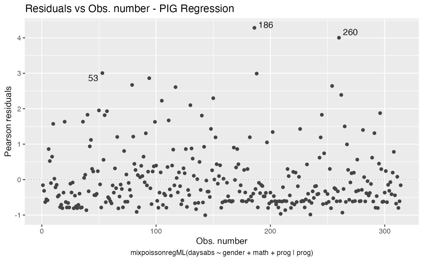
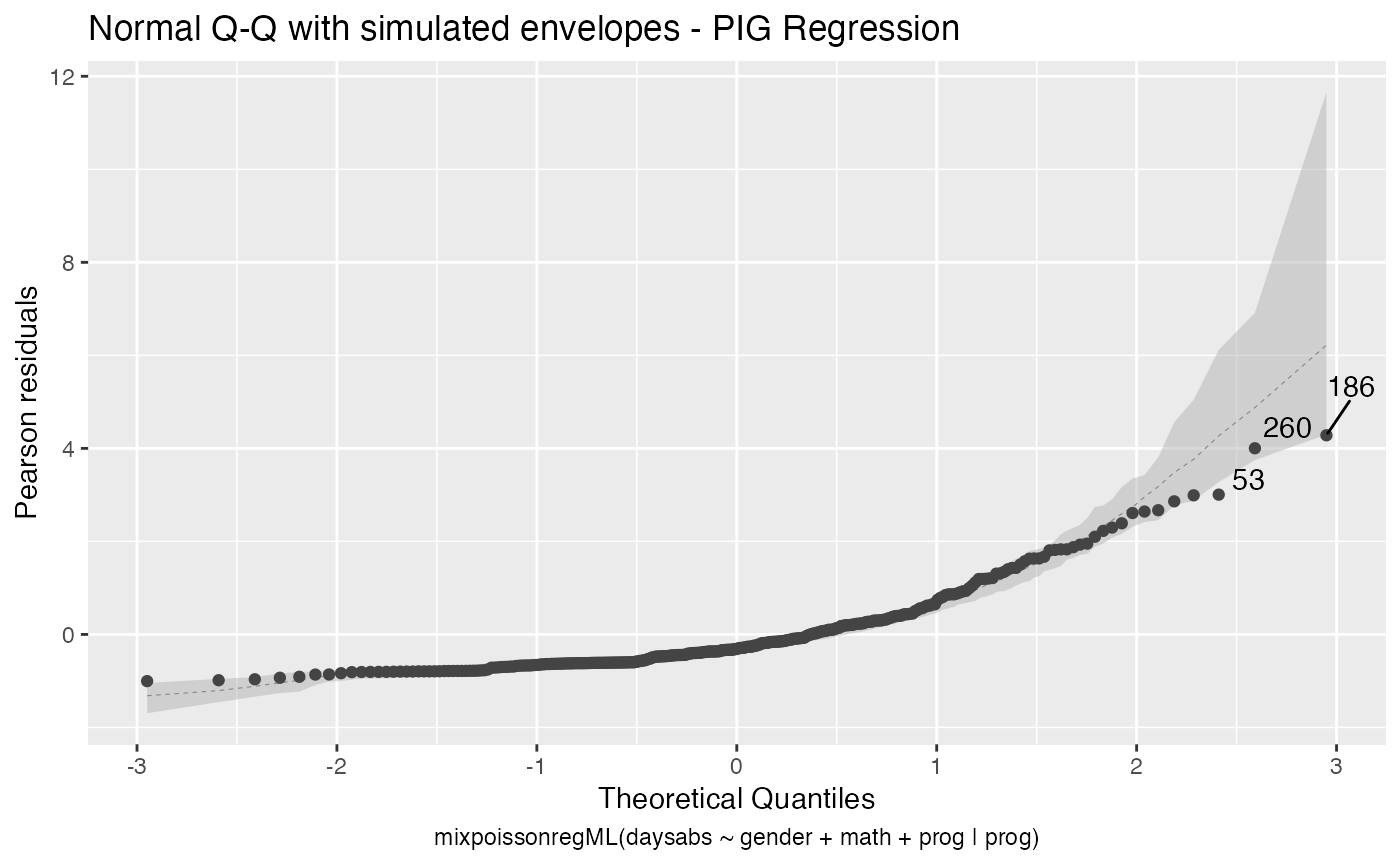
Notice that in Residuals vs. Obs. number, the residuals appear to be randomly distributed, skewed, and with no noticeable trend. Thus, also suggesting an adequate fit, together with the quantile-quantile plot with simulated envelopes.
Influence analysis
Let us begin with the global influence analysis. First, for the NB regression model:
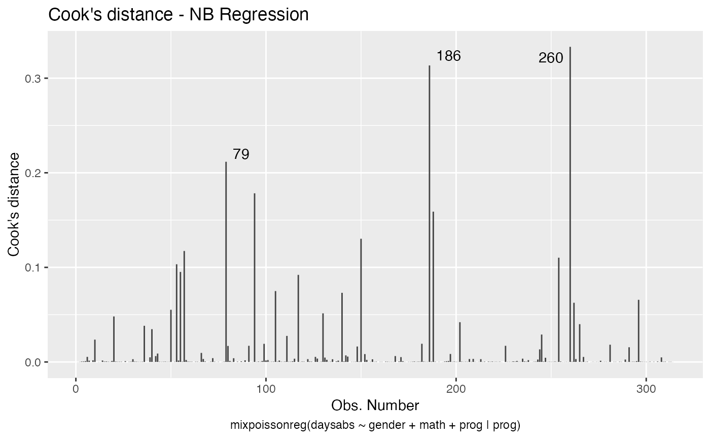
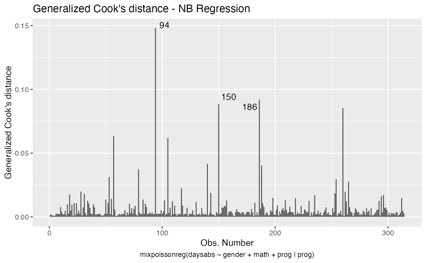
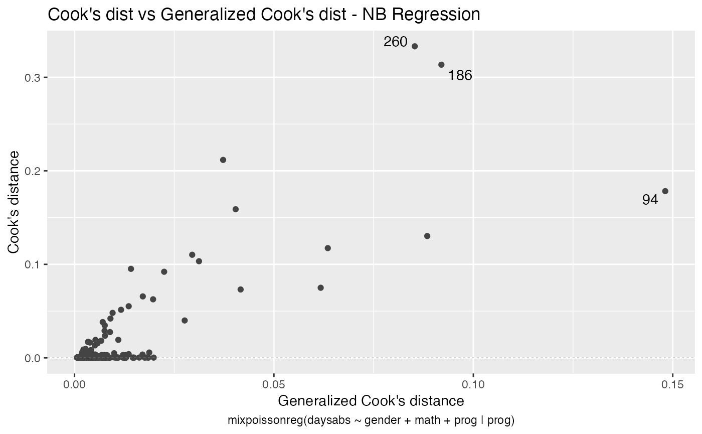
Second, for the PIG regression model:
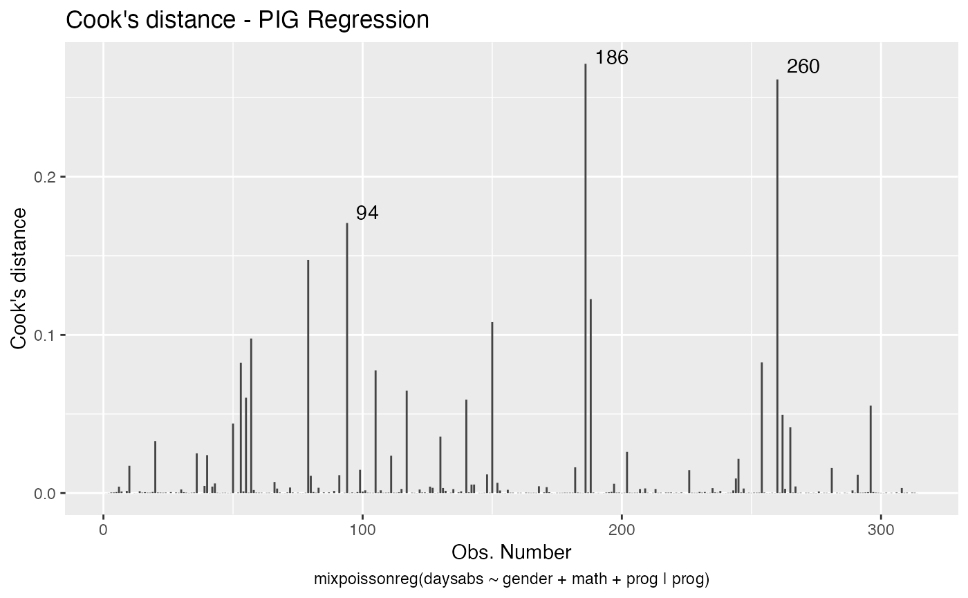
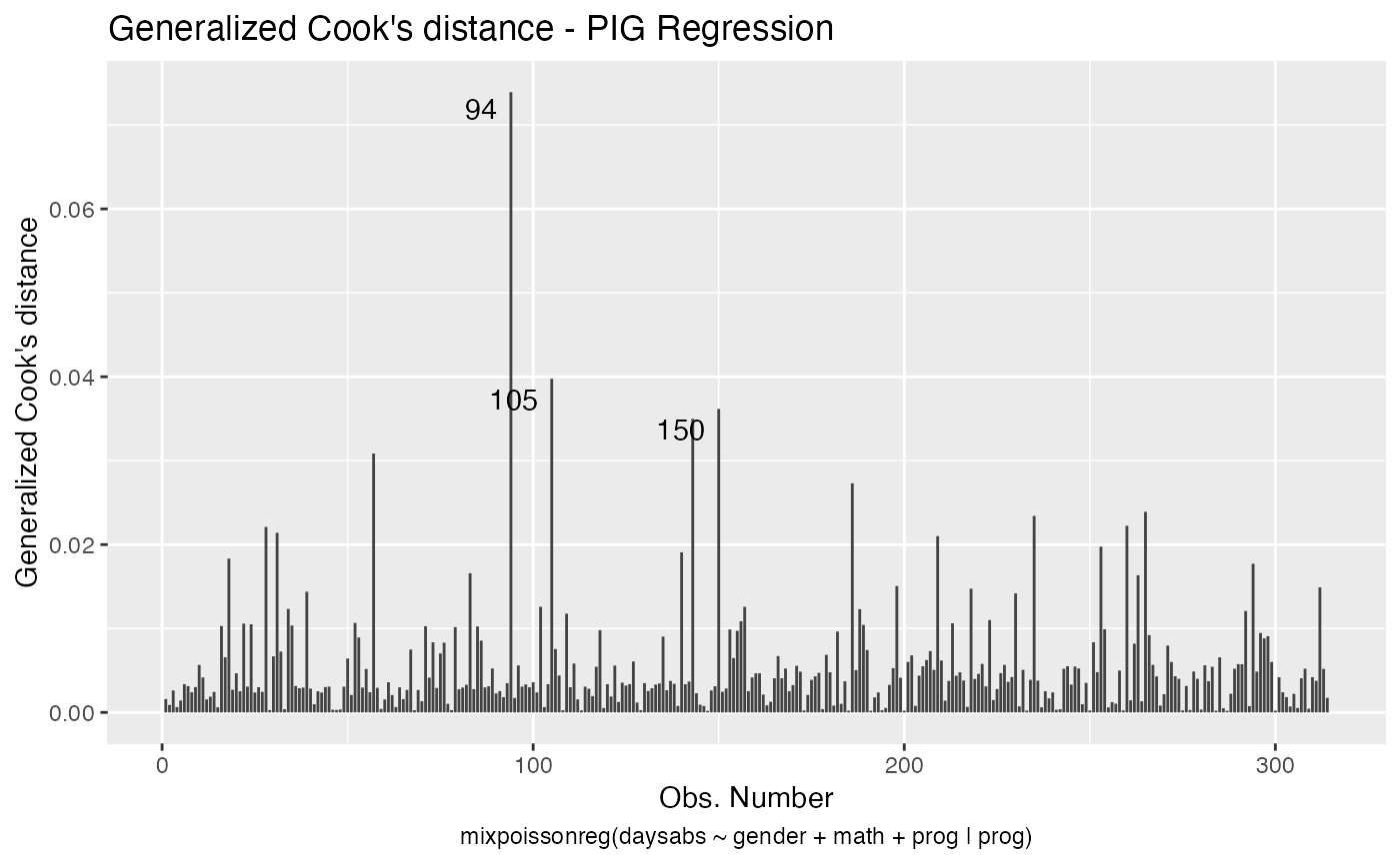
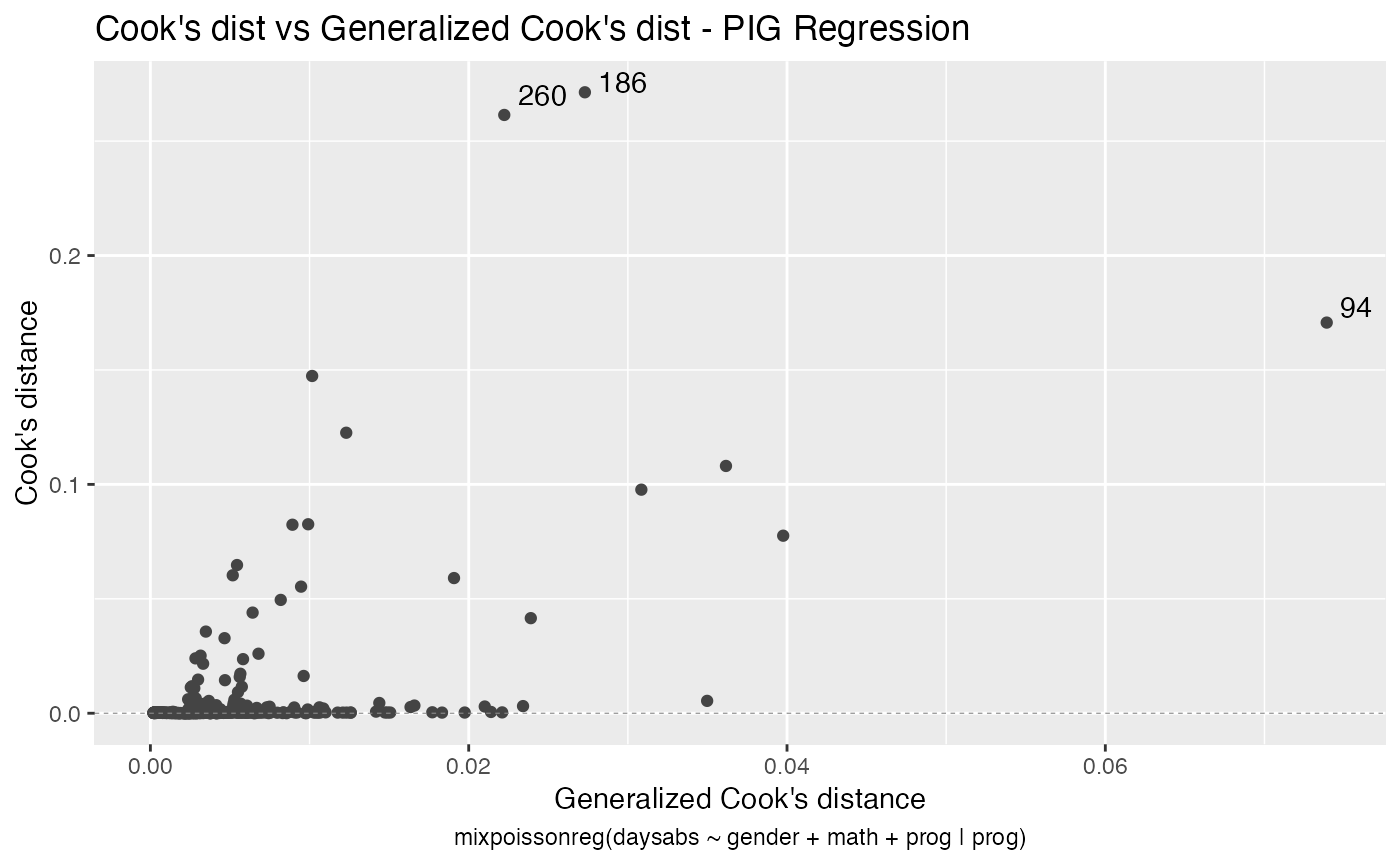
Let us check the impact on the estimates of the removal, for example, of case # 94, which was significant for both models, as well as it was the most significant considering both the Cook’s distance and generalized Cook’s distance. First, for NB regression:
# Relative change for mean-related coefficients
(influence(fit_nb_red)$coefficients.mean[94,] -
   coefficients(fit_nb_red, parameters = "mean"))/
  coefficients(fit_nb_red, parameters = "mean")
#>    (Intercept)     gendermale           math   progAcademic progVocational
#>   -0.002673517   -0.012802496    0.017218704   -0.024328409   -0.010166827

# Relative change for precision-related coefficients
(influence(fit_nb_red)$coefficients.precision[94,] -
    coefficients(fit_nb_red, parameters = "precision"))/
  coefficients(fit_nb_red, parameters = "precision")
#>    (Intercept)   progAcademic progVocational
#>     0.05296451     0.05422589     0.03873275
Now, for the PIG regression:
# Relative change for mean-related coefficients
(influence(fit_pig_red)$coefficients.mean[94,] -
   coefficients(fit_pig_red, parameters = "mean"))/
  coefficients(fit_pig_red, parameters = "mean")
#>    (Intercept)     gendermale           math   progAcademic progVocational
#>   -0.001926543   -0.008484376    0.011185047   -0.018039686   -0.007642806

# Relative change for precision-related coefficients
(influence(fit_pig_red)$coefficients.precision[94,] -
    coefficients(fit_pig_red, parameters = "precision"))/
  coefficients(fit_pig_red, parameters = "precision")
#>    (Intercept)   progAcademic progVocational
#>     0.04511006     0.03269834     0.02399582
We see that case # 94 mainly impacts the precision parameter estimates. Notice that for PIG regression models, the impact is less severe.
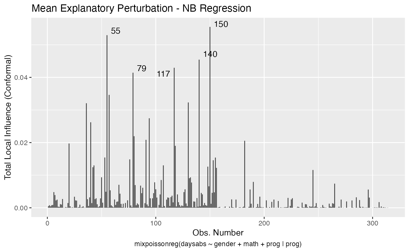
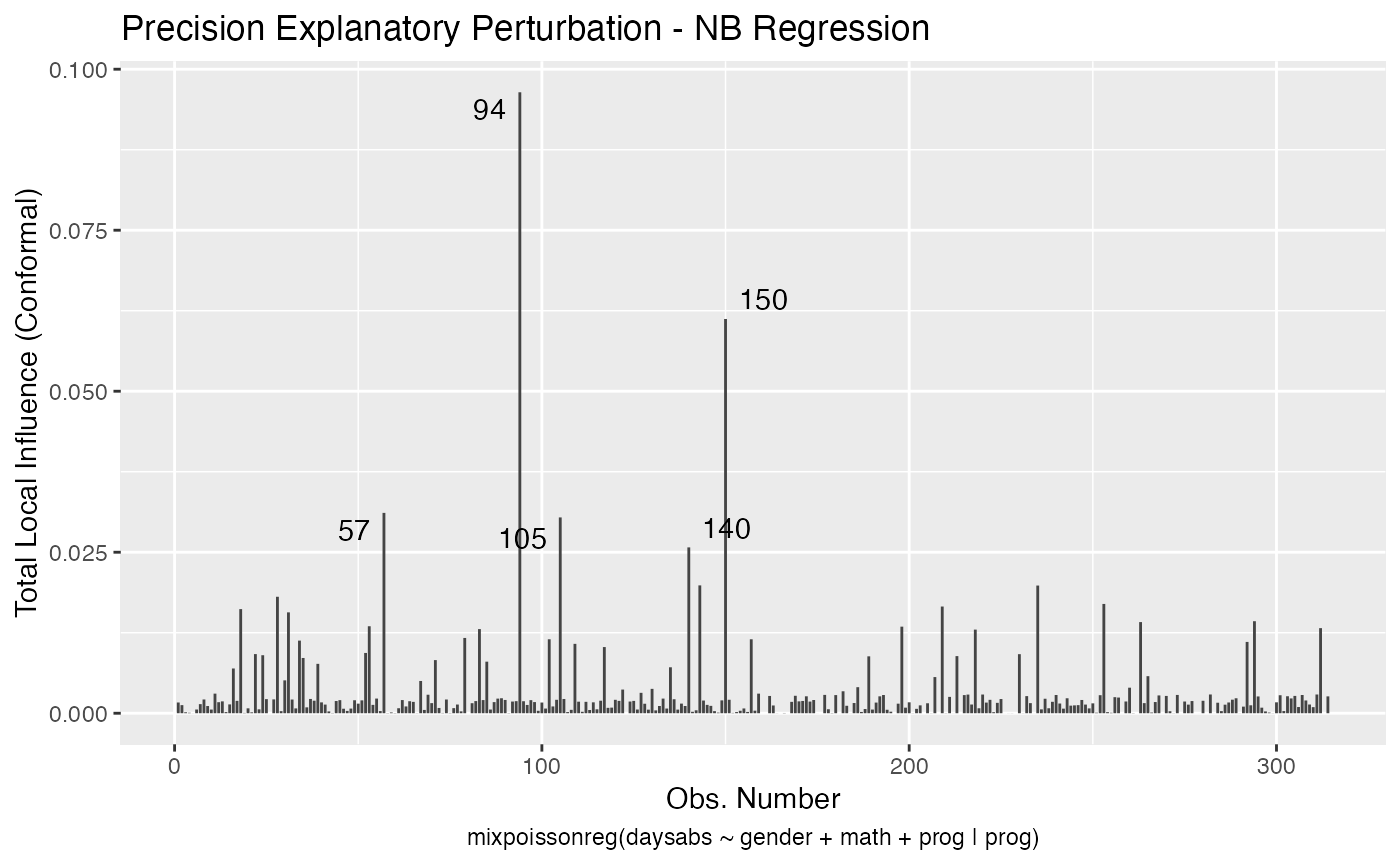
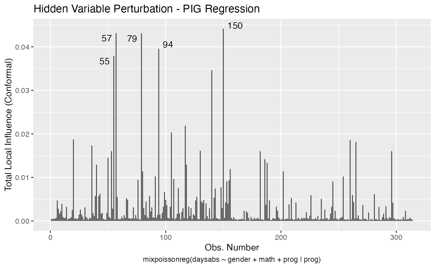
Let us check now the local influence.
First for the NB regression:
local_influence_autoplot(fit_nb_red)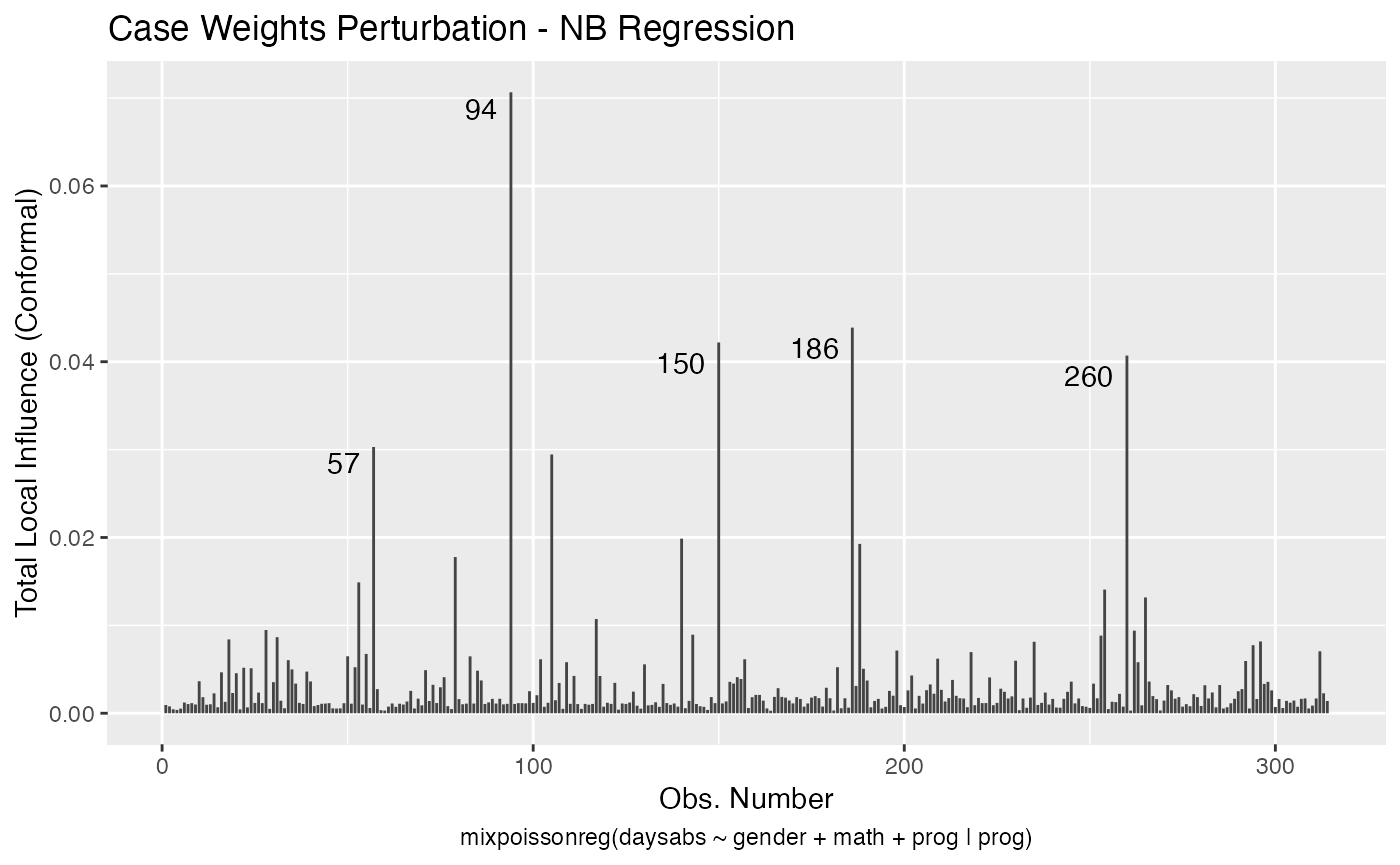
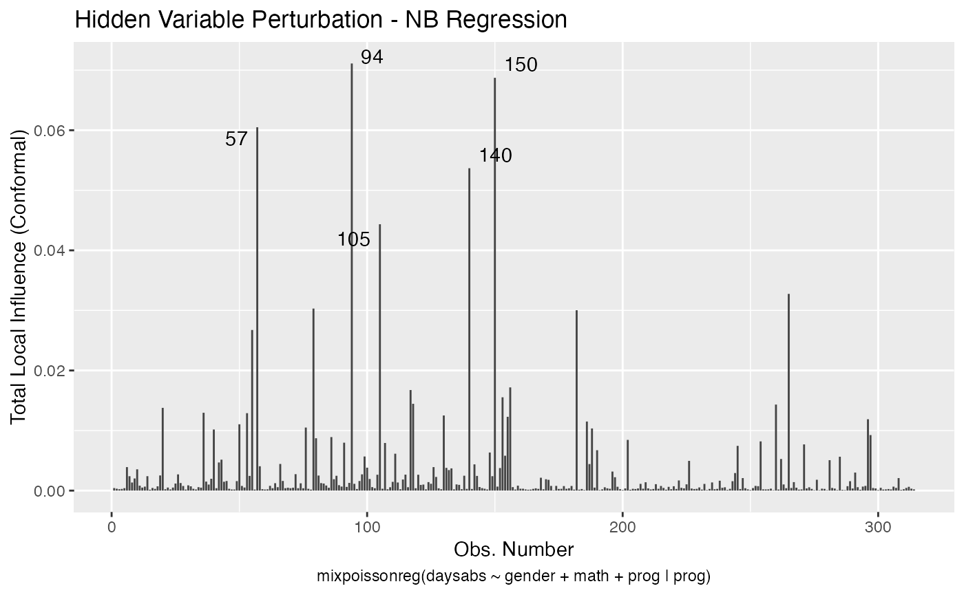
Now, for PIG regression:
local_influence_autoplot(fit_pig_red)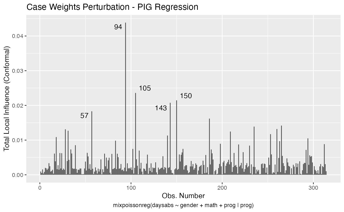
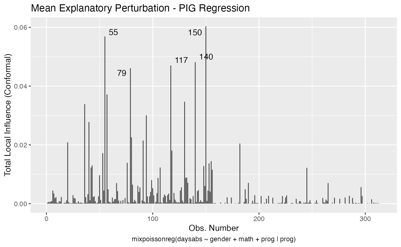
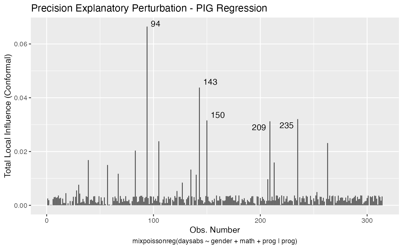
Let us check the influential observations along with their associated covariates and response values. First for the NB regression:
inf_nb_tbl <- tidy_local_influence(fit_nb_red) %>% mutate(.index = row_number()) %>%
  pivot_longer(!.index, names_to = "perturbation", values_to = "curvature")
bench_nb_tbl <- local_influence_benchmarks(fit_nb_red) %>%
  pivot_longer(everything(), names_to = "perturbation", values_to = "benchmark")

inf_nb_bench_tbl <- left_join(inf_nb_tbl, bench_nb_tbl, by = "perturbation") %>%
  mutate(influential = curvature > benchmark) %>% filter(influential == TRUE) %>%
  select(-influential, -benchmark, -curvature)

data_nb_tbl <- augment(fit_nb_red) %>% mutate(.index = row_number()) %>%
  select(.index, daysabs, gender, math, prog)

influential_nb <- left_join(inf_nb_bench_tbl, data_nb_tbl, by = ".index")

influential_nb
#> # A tibble: 55 x 6
#>    .index perturbation             daysabs gender  math prog
#>     <int> <chr>                      <dbl> <fct>  <dbl> <fct>
#>  1     20 mean_explanatory              24 male       4 Academic
#>  2     20 simultaneous_explanatory      24 male       4 Academic
#>  3     36 mean_explanatory              28 female    20 Academic
#>  4     36 simultaneous_explanatory      28 female    20 Academic
#>  5     40 mean_explanatory              27 female    35 Academic
#>  6     40 simultaneous_explanatory      27 female    35 Academic
#>  7     55 hidden_variable               34 female     4 Academic
#>  8     55 mean_explanatory              34 female     4 Academic
#>  9     55 simultaneous_explanatory      34 female     4 Academic
#> 10     57 case_weights                  28 male       5 General
#> # … with 45 more rows
Let us check the number of unique influential observations:
influential_nb %>% select(.index) %>% unique() %>% count()
#> # A tibble: 1 x 1
#>       n
#>   <int>
#> 1    22
Now for the PIG regression:
inf_pig_tbl <- tidy_local_influence(fit_pig_red) %>% mutate(.index = row_number()) %>%
  pivot_longer(!.index, names_to = "perturbation", values_to = "curvature")
bench_pig_tbl <- local_influence_benchmarks(fit_pig_red) %>%
  pivot_longer(everything(), names_to = "perturbation", values_to = "benchmark")

inf_pig_bench_tbl <- left_join(inf_pig_tbl, bench_pig_tbl, by = "perturbation") %>%
  mutate(influential = curvature > benchmark) %>% filter(influential == TRUE) %>%
  select(-influential, -benchmark, -curvature)

data_pig_tbl <- augment(fit_pig_red) %>% mutate(.index = row_number()) %>%
  select(.index, daysabs, gender, math, prog)

influential_pig <- left_join(inf_pig_bench_tbl, data_pig_tbl, by = ".index")

influential_pig
#> # A tibble: 64 x 6
#>    .index perturbation             daysabs gender  math prog
#>     <int> <chr>                      <dbl> <fct>  <dbl> <fct>
#>  1     20 hidden_variable               24 male       4 Academic
#>  2     20 mean_explanatory              24 male       4 Academic
#>  3     20 simultaneous_explanatory      24 male       4 Academic
#>  4     28 case_weights                   0 female    21 Academic
#>  5     31 case_weights                   0 male       1 Academic
#>  6     36 hidden_variable               28 female    20 Academic
#>  7     36 mean_explanatory              28 female    20 Academic
#>  8     36 simultaneous_explanatory      28 female    20 Academic
#>  9     39 precision_explanatory          5 male       1 General
#> 10     40 mean_explanatory              27 female    35 Academic
#> # … with 54 more rows
Now, the number of unique influential observations for the PIG regression:
influential_pig %>% select(.index) %>% unique() %>% count()
#> # A tibble: 1 x 1
#>       n
#>   <int>
#> 1    28
Let us check the informations of case # 94 for the NB and PIG regressions:
influential_nb %>% filter(.index == 94)
#> # A tibble: 5 x 6
#>   .index perturbation             daysabs gender  math prog
#>    <int> <chr>                      <dbl> <fct>  <dbl> <fct>
#> 1     94 case_weights                  29 female    70 General
#> 2     94 hidden_variable               29 female    70 General
#> 3     94 mean_explanatory              29 female    70 General
#> 4     94 precision_explanatory         29 female    70 General
#> 5     94 simultaneous_explanatory      29 female    70 General

influential_pig %>% filter(.index == 94)
#> # A tibble: 5 x 6
#>   .index perturbation             daysabs gender  math prog
#>    <int> <chr>                      <dbl> <fct>  <dbl> <fct>
#> 1     94 case_weights                  29 female    70 General
#> 2     94 hidden_variable               29 female    70 General
#> 3     94 mean_explanatory              29 female    70 General
#> 4     94 precision_explanatory         29 female    70 General
#> 5     94 simultaneous_explanatory      29 female    70 General
So, notice that case # 94 is a female, enrolled in the general program, with a high number of absences but with an unexpected high math score for this number of absences.
It is also noteworthy that case # 94 was considered influential for all local perturbation schemes.
Let us check the observations that were found influential for both models:
ind_nb <- influential_nb %>% select(.index) %>% unique()

ind_pig <- influential_pig %>% select(.index) %>% unique()

ind_common <- intersect(ind_nb, ind_pig)

influential_nb %>% filter(.index %in% ind_common$.index) %>% select(-perturbation) %>% unique()
#> # A tibble: 20 x 5
#>    .index daysabs gender  math prog
#>     <int>   <dbl> <fct>  <dbl> <fct>
#>  1     20      24 male       4 Academic
#>  2     36      28 female    20 Academic
#>  3     40      27 female    35 Academic
#>  4     55      34 female     4 Academic
#>  5     57      28 male       5 General
#>  6     79      35 male       1 Academic
#>  7     80      23 female    21 Academic
#>  8     91      23 female    27 Academic
#>  9     94      29 female    70 General
#> 10    105      19 male      70 General
#> 11    117      35 female    35 Academic
#> 12    130      30 female    34 Academic
#> 13    140      30 female    27 General
#> 14    143       5 female     7 General
#> 15    150      34 female    29 General
#> 16    182      21 female    47 General
#> 17    186      16 male      81 Vocational
#> 18    235       3 female    67 General
#> 19    260      19 male      49 Vocational
#> 20    265      16 female    99 General
Now, let us check the influential observations for the NB regression that were not influential for the PIG regression:
ind_nb_pig <- setdiff(ind_nb, ind_pig)

influential_nb %>% filter(.index %in% ind_nb_pig$.index) %>% select(-perturbation) %>% unique()
#> # A tibble: 2 x 5
#>   .index daysabs gender  math prog
#>    <int>   <dbl> <fct>  <dbl> <fct>
#> 1    118      16 female     8 General
#> 2    188      16 female    75 Vocational
Finally, the influential observations for the PIG regression that were not influential for the NB regression:
ind_pig_nb <- setdiff(ind_pig, ind_nb)

influential_pig %>% filter(.index %in% ind_pig_nb$.index) %>% select(-perturbation) %>% unique()
#> # A tibble: 8 x 5
#>   .index daysabs gender  math prog
#>    <int>   <dbl> <fct>  <dbl> <fct>
#> 1     28       0 female    21 Academic
#> 2     31       0 male       1 Academic
#> 3     39       5 male       1 General
#> 4     83       3 female    84 General
#> 5    209       4 female    41 General
#> 6    213       4 female    63 General
#> 7    253       0 female    29 Academic
#> 8    263       3 male      43 General